
Estimating Combined Variance from Sub Groups
Background
I have millions of domestic bin lift records which need to be processed in two ways:
Firstly they need statistics generated for each bin, including mean location and variance of location;
Secondly they need statistics generated for the premises that they belonged to.
With millions of records this process was becoming too lengthy and a quicker approach needed to be taken. I was able to create a means by which variance of bin collections at the premises could be estimated from the variance of each bin's collection data. The fact that the data is bins is not relevant, so from this point forward I will relate to the bin collection clusters as "Sub-samples" (of a premises collection data) and all collection data for the premises as "sample". The total population of collections for the premises include future collections - and therefore can only be temporally sub-sampled.
A number of sub-samples are taken of the same populations. Each sub-sample has its own mean and variance. There are some 60,000 separate populations, with each normally having 2-3 sub-sample groups, and rarely as many as a dozen sub-sample groups. Each sub-sample group may have many hundred data points. Using all the data from each sub-sample to calculate a combined sample Variance and mean was taking too long. Therefore a new approach was required. In the end I think all I have created a geometric proof of the "Law of Total Variance" - however I don't have the formal mathematics education to be sure.
The new sample mean and Variance are to be estimated from the aggregate data of the sampled groups rather than a recomputation of the combined data. This will cut calculation time down many times over.
It can be assumed the data is normally distributed on the X and Y axis, and have the same deviation in both X and Y axes.
The new sample mean (centroid) is calculated as the weighted average of the sub-sample means.
The new variance estimate for each group is based on the current variances of the sub-groups with the addition of the squared average distance to the new mean (thus increasing the current variance by the square of the average distance). Therefore, if all sub-sample variances and mean centroids are the same, the values don't change, but if there is a difference between means, the variance is increased proportional to the size (number of data points), current variance and distance of the sub-sample from the new centroid. It is not expected that the process will be perfectly accurate but rather a solid estimate within a couple of percent.
Theory
The theory begins by determining the average distance to the circumference of circle. A circle is being used because variance can be represented as a circle around the data.
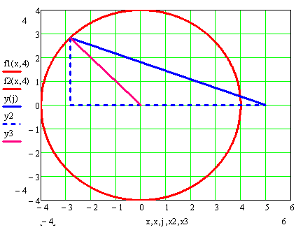
Figure 1: Distance of a circle to a specifici point
From Figure 1 above we can see that the aim is to find the length of the blue hypotenuse (H)
To do this We need to know the two other sides of the triangle (blue dotted lines).
Take the left most vertical line to be "Y", the portion of the dotted X axis below the pink line as "X" and the length of the pink line to be "R" (radius).
The distance from the far left point to the centre of the circle is D
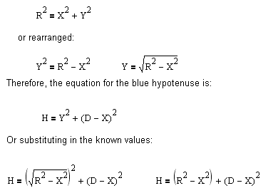
The same equation holds when the distance is on the other side of the circle, as shown in Figure 2:
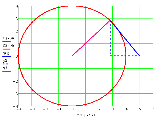
Therefore, given radius r and distance to centre of circle d, the distance at any point along the circle is:

However, this is only one distance and we need the average distance. All distances between all points along the circumference of the circle and the the "distant" coordinate can be determined through integration.
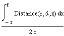
When there is no difference in distance between the coordinate and the centre of the circle the average distance to the circumference of the circle is the radius.
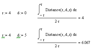
Therefore - the average distance to the perimeter of a circle with radius 4 and the distance to the centre of the circle is 5 is 6.067
This provides us with the distance function:
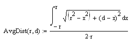
This is the average distance from the circumference of a circle to a specific point.
The difference between the distance to the centroid of the circle and the average distance the the perimeter is explained by angles. From the images above, the distance of the 45 degree data point closest to the "P" data point is far larger compared to the x-axis distance than the distance to the furthest 45 degree data point compared to its x-axis distance. This is due to the steep angle of the close 45 degree data point compared to the smaller angle of the further 45 degree data point. If D were greater the difference in the angles for both the 45 degree data points would be less, and therefore the proportional difference between them would reduce.
Thus, as D increases the effect of the the average distance approaches the the distance to the centre of the circle.
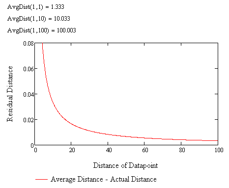
The greatest effect is therefore found when the distance is "close" (proportionally close as a ratio to the radius). The goal of this exercise is to create a new variance based on multiple samples which will therefore have close values. Therefore these distance calculations are pivotal to this exercise.
Variance Calculation
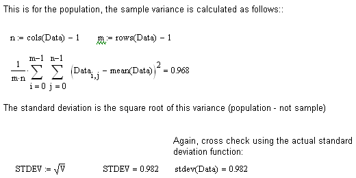
Firstly I'll create a set of test data, using a normal distribution with standard deviation of 1. The variance to a specific coordinate can both be estimated and measured. Variance can be interpreted as a distance measure, measuring the mean squared distance from the data centroid (population - not sample) divided by the dimensions.
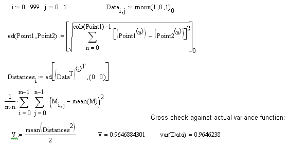
Variance Estimation
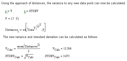
Normally when calculating out a new variance all sub-samples would be combined. Instead this example will use only one sub-sample's contribution - so this is the partial effect of the sub-sample on the new sample data. Normally the variance calculation id quite simple but requires every data-point to be used when computed. The goal is to create a simpler way of generating the same partial effect value as this calculation.
If we use the sub-sample variance as the radius of a circle we simply need to estimate the additional distance that would be added to this circle by the new centroid location. This is done by adding the square of the average distance.
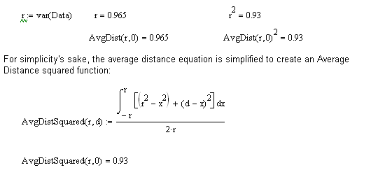
There are two complicating issues, both relating to the fact we are using the mean of "squared distances" rather than the "mean distances" squared.
Firstly the mean distance squared is calculated as half the average squared distance. This allows us to measure the distance added to the base variance of the data.
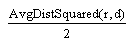
We are interested in the additional distance added to the variance, and therefore we must factor in the underlying variance to the current centroid while removing the average squared distance measuremet from the centre of the circle.
For instance, the estimate value should equal the actual variance when the distance away from the variance is zero.
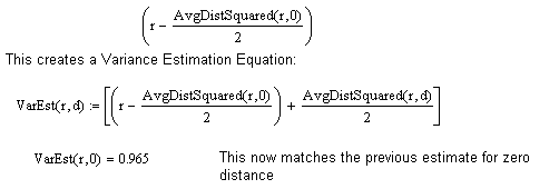
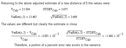
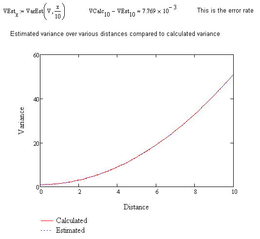
This is designed to be a close estimate. That is, The difference between the actual variance and the estimated variance will has a specific but small error rate.
The error rate is introduced through the assumption that the data is perfectly normally distributed, thus having an even variance in both axes, if that is not the case (which is likely with sample measures), the variance in every direction is not perfectly even thus causing an error in the calculation. Thus the smaller the sample size, the larger this error is.
This error rate magnifies linearly with distance along a specific vector. Thus at small distances the error rate is low while at larger distances it is large, but the error amount remains proportion to distance. Therefore it is possible to eliminate this error by calculating the error rate over a specified distance along a specific vector and then adding a correcting factor for all future distances, but multiple distances aren't important to this endeavour.
As the very purpose of the measure is to combine variances that are close distances to each other, the error is always minimised and therefore acceptable.
Standardised Approach
The goal of this exercise is to reduce computation and the inclusion of integration in the process is likely to increase computation time. That is, the estimate will take longer to computer than simply using all data for an accurate measure or using the Law of Total Variance. To resolve this issue a simplified function based on a standardised (normalised) variance is used. This is as follows:
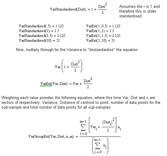
Thus a very simple equation can be used to determine the sample variance based on sub-sample variances without any need to transform the data and without any complicated calculations.